
How many games will our team win?
The 2005-06 Boston Celtics posted a 33-49 win-loss record, winning only 40% of their games, and heading into the next season, they were about to hit rock bottom.
If we were Celtics fans (or critics) at the beginning of that terrible 2006-07 season, what would we have predicted their upcoming win percentage to be?
There are many factors that we might have used to arrive at our prediction. We might have surveyed fans, read sportswriters’ opinions, or guessed at how players’ current health would affect the team’s performance. But for our purposes, we’re going to keep things simple and use the team’s 2005-06 win percentage as our prediction for the 2006-07 season.
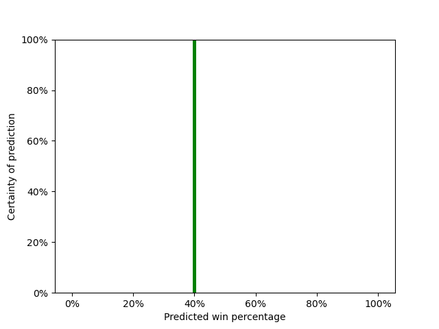
The plot above shows our prediction of 40%. But are we absolutely sure that the Celtics will win exactly 40% of their games? Well, no. Maybe they’ll win only 35%. Maybe they’ll win 45%, or even improve all the way past 50%.
How (Un)Certain are we?
We can think about our certainty or uncertainty as if each win percentage has its own probability of coming true. If we’re absolutely sure that the Celtics will win 40% of their games, as in the plot above, then we’re 100% certain that the Celtics will win 40% of their games.
But maybe we’re less certain than that. Maybe we’re 100% certain that the Celtics will win between 38% and 42% of their games. Our prediction might be represented by the plot below.
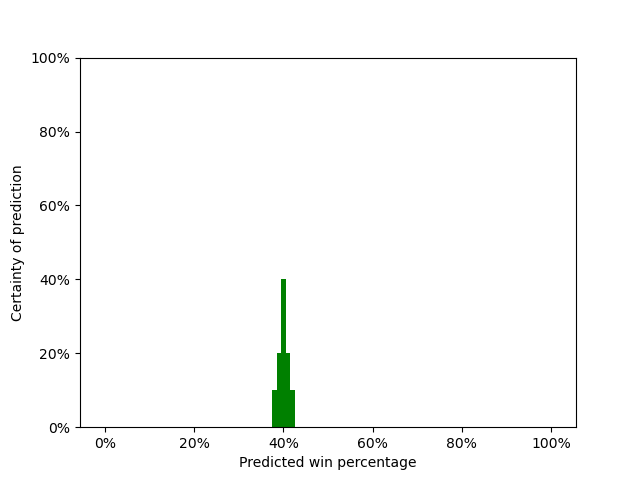
In this plot, we’re saying that we’re 10% sure that the Celtics will win 38% of their games, 20% sure that they’ll win 39%, 40% sure that they’ll win 40%, 20% sure that they’ll win 41%, and 10% sure that they’ll win 42%.1
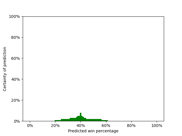
Or we might be even less certain than that. The plot below still shows that our most likely prediction for the Celtics’ win percentage is 40%, but we’re allowing for a much wider range of possibilities – that is, we’re much less certain than we were before.
Transform certainty into math
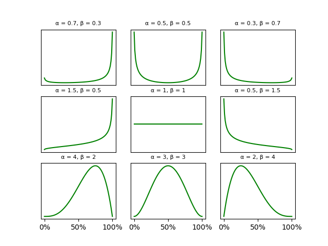
Up to this point, we’ve avoided using any statistical jargon, but now is a good time to introduce the beta distribution. The beta distribution ranges from zero to one (or 0% to 100%), and we can use it to model probabilities of probabilities, like our (un)certainty about the Celtics’ predicted win percentage. Here are some examples of what the beta distribution can look like for some selected values of its parameters, α (alpha) and β (beta).2
In our case, we think that the best prediction for the Celtics’ win percentage next season is the same as their actual win percentage for this past season: 40%. So we can make 40% be the peak (or, the mode) of our beta distribution. We can calculate the mode of the distribution from its parameters, so we want parameters that satisfy this equation:
Next, we need to decide how narrow (certain) or wide (uncertain) our beta distribution should be. There are many ways we could do this. One way is to consider how likely a team with a 40% win percentage from last season is to have a winning season (i.e., win percentage > 50%) next season. We could look at historical NBA statistics and see how many teams had achieved that before the 2005-06 season. Or we could keep things simple and guesstimate based on our honed basketball intuitions: let’s say 35%.
Altogether, we want parameters for the beta distribution where the mode is 0.40 and the area under the beta curve where x > 0.50 is 0.35. It turns out that the parameters α = 2.85 and β = 3.775 give us this approximate result. Here’s what that distribution looks like:
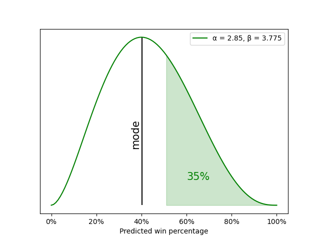
That distribution represents our belief at the beginning of the 2006-07 season about how much the Boston Celtics will win: we think that it’s most likely that the Celtics will win 40% of their games and that they will probably have a losing season, but we’re giving them a 35% chance that they’ll win more games than they lose.
How do we update our predictions after one game?
Now suppose Boston loses their first game of the 2006-07 season (they did). Surely that should decrease our prediction that they’ll most likely win 40% of their games, right? But by how much? And likewise, surely we’ll now predict that their chances of having a winning season are lower than 35%, right? But again, by how much?
We could guesstimate again, but we actually have a convenient mathematical model that can update our prediction quite elegantly: the beta-binomial model. In this model, we start with our beta distribution, which represents our initial belief. Then we get some binomial data: did the team win or lose? That tells us how to update our beta distribution. In fact, the update rule is remarkably simple: we add one to the appropriate beta distribution parameter. That gives us our new beta distribution, which represents our new prediction after that first game finishes.
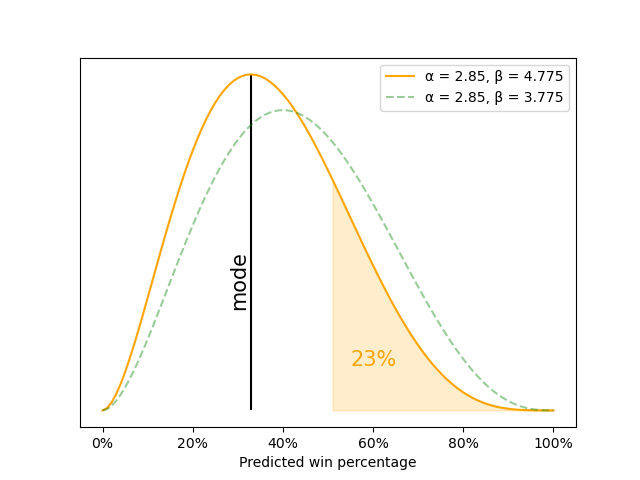
For the start of the 2006-07 Celtics season, we started with a beta distribution with α = 2.85 and β = 3.775. Boston lost, so we add one to β: 3.775 + 1 = 4.775. That gives us a new beta distribution where α = 2.85 and β = 4.775. The mode of this new distribution is:
And this new distribution gives the Celtics only a 23% chance of finishing their season with a winning record. We can see this new, updated beta distribution in the plot below:
How do we update our predictions after many games?
We don’t have to stop updating at a single game. For every game that the Celtics play, we can generate a new update using the same beta-binomial model. We simply cycle through the same steps for every game:
- we start with a beta distribution that represents our current belief about how often the Celtics win games,
- we observe whether the team wins or loses the next game, and
- we use that win-loss binomial data to update our starting beta distribution to our new beta distribution.
To re-start the cycle, the updated beta distribution for one game becomes the starting distribution for the next game’s update.
When we do all the updates across the Celtics’ 2006-07 season, our series of beta distributions looks like this:3
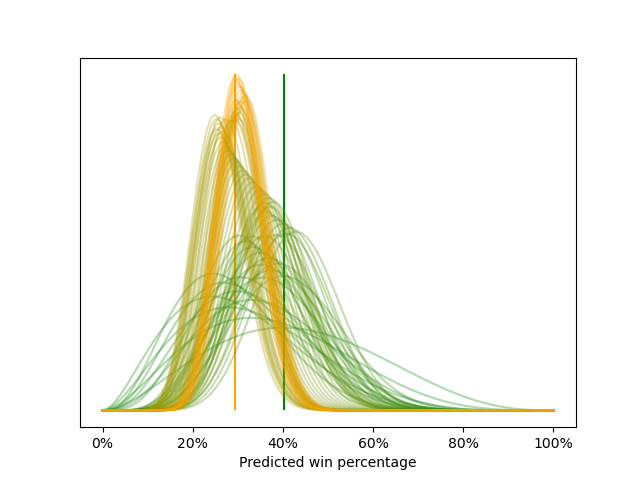
The plot above shows that our starting beta distribution has a peak at the prior season’s final win percentage of 40% (marked by the vertical green line), and it is wide, which shows our uncertainty about our belief. As the season progresses and we add more game data, our beta distributions shift toward the current season’s final win percentage (29%, marked by the vertical yellow line) with more and more certainty (i.e., narrower and narrower distributions).
Below is an animation of the same series of beta distributions.
What if our starting distribution is a poor estimate?
Across the Celtics’ 2006-07 season, our best estimate of the Celtics’ win percentage shifts from 40% to 29% and becomes more and more certain. But 40% and 29% are not far apart; in other words, our starting estimate of 40% was fairly good, because it was fairly close to the final estimate of the season. But what happens when that starting estimate isn’t that good?
To find out, let’s apply the same kind of analysis to the next Celtics season: the 2007-08 season. This season marked an astounding recovery for Boston, as they transformed from one of the worst teams in the league in the prior season to the best one.
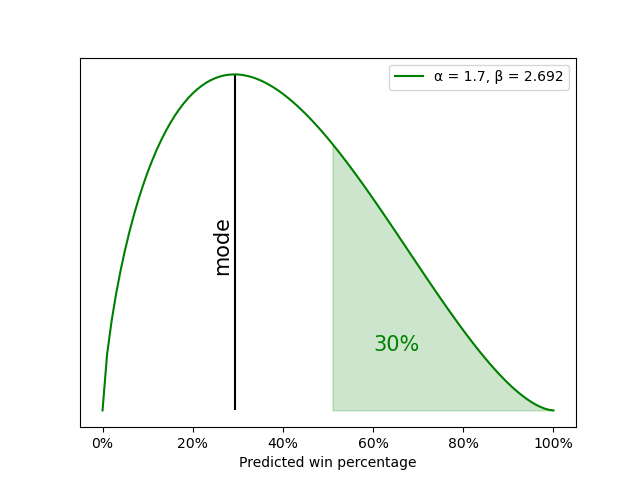
Let’s set up a starting beta distribution for the 2007-08 season based on the Celtics’ performance in the 2006-07 season when they won 29% of their games. The peak of our beta distribution, then, is 29%, and we’ll guesstimate that such a team has a 30% of having a winning record. A beta distribution with α = 1.7 and β = 2.692 gives us our desired characteristics, as shown below.
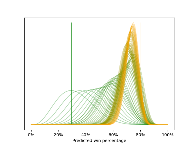
When we start with the beta distribution above and update it for every game of the Celtics’ 2007-08 season, we get the series of beta distributions shown below.
Notice that the beta distributions quickly shift from low win percentages to high win percentages as the Celtics win their first several games of the season. Also notice that the final beta distribution peaks very close to the final season win percentage of 80% (as marked by the yellow vertical line).
Below is an animation of the same series of beta distributions.
What if we’re too confident about our poor estimate?
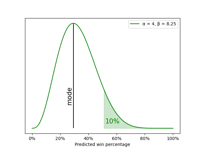
What happens to the updates if we’re more confident at the start of the 2007-08 season that the Celtics will have another bad season? In the example above, we gave the Celtics a 30% chance of having a winning season. What if we gave them only a 10% chance? Let’s start with a beta distribution with α = 4 and β = 8.25, which provides a peak at 29% and a 10% chance that the Celtics will win more than half their games.
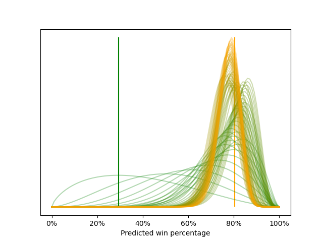
When we start with this more confident beta distribution above and update it for every game of the Celtics’ 2007-08 season, we get the series of beta distributions shown below.
Below is an animation of the same series of beta distributions.
Notice that it now takes many games for the beta distributions to shift from low to high win percentages. This illustrates an important point: if we start with a confident distribution and we’re wrong, it takes a lot of data to adjust our estimates. This slow shift contrasts with our previous example, when we started with a much less confident beta distribution (giving Boston a 30% chance of having a winning season, instead of a 10% chance), and our updates shifted much more quickly.
Statisticians often advise us to start with distributions that are somewhat less confident than we think they should be. There is usually little to gain from having an overly confident distribution that turns out to be quite accurate: usually, we get a modestly higher probability that the ultimately-correct estimate is correct.4 But the cost to having an overly confident distribution that is inaccurate can be severely high: it might make one ignore a real possibility that ultimately comes true, or it might make one slow to adapt to the surprisingly different situation.
Notes
1Yes, there were fewer than 100 games in the 2006-07 season, so I’m ignoring that the actual possible distribution is not that smooth. Its resolution is >1% and the possible percentages don’t fall exactly on the percentiles.
2Keep in mind that the beta distribution isn’t the only way to model probabilities of probabilities. For example, the beta distribution has only one or two peaks (or, in jargon, modes), but perhaps your knowledge and certainty about basketball requires three or four or more peaks. Or maybe it requires a discontinuous function.
3Two caveats:
First, our beta-binomial model assumes that the Celtics’ actual win percentage is constant across the entire season. Each new observation of data – each game – simply brings our estimate closer and closer to that true win percentage. However, in a real basketball season, a team’s chance of winning may vary depending on how good the opponent is, playing at home vs. away, team members’ injuries, etc. As we mentioned previously, this a simple model.
Second, we technically changed the problem a bit. We started saying that we want to predict the Celtics’ win percentage for the season. But at the end of the season, we know exactly what the final win percentage is, even though our estimate still shows some uncertainty (and its mode might not even equal the final win percentage, depending largely on the prior that we start with). Really, what our model is doing is estimating that “true” win percentage; the actual win percentage that we observe might not exactly match the “true” win percentage because of some random events that show up in our data. The “true” win percentage is like estimating the team’s “strength”: we can’t see “strength” directly, because it’s an abstract concept. But we can see its effects in our data. We’ve been glossing over this technical point, because our primary focus is to convey general concepts about the beta-binomial model and the dynamics of how it updates.
4Or, for all us jargon-lovers, our credible intervals are narrower and still contain the true value of the estimated parameter.
The code for the Plotly Dash app that runs the beta distribution updates shown in the videos can be found here.