If you prefer a prettier rendering of the code and dataframes displayed in this article, you are welcome to read the notebook at my Github repo.
How fast is Polars for realistic data processing jobs?
The dataframe library Pandas has long been a
workhorse for data scientists, ML engineers, and other data professionals.
It has a broad, convenient, user-friendly API for transforming and
summarizing data, which allows us to quickly discern insights from our data
and engineer data pipelines for production. But how quickly, exactly? A
new dataframe library Polars claims to be much
faster at processing data than Pandas
and other common tools.
I was curious about how much faster Polars might be not only on benchmarks but also as part of realistic data workflows. So, I created some data to be processed by Pandas or Polars. Since file-reading is typically among the slower parts of a data pipeline, I stored the data in either the older, ubiquitous comma-separated-values (CSV) format or the newer, column-based Parquet format. Additionally, Polars can be used from either Python or Rust, so comparing the workflow in those two languages would be useful. Finally, Polars jobs can be processed eagerly or lazily, so we can compare both execution approaches in our workflow.
To summarize, we’ll compare:
- Pandas vs. Polars
- Python Polars vs. Rust Polars
- CSV vs. Parquet
- Polars Eager vs. Polars Lazy
For each comparison pair in the list above, the bolded variation is the one I expected to be faster. That is, I expected Polars to be faster than Pandas, Rust to be faster than Python, Parquet to be faster than CSV, and Lazy to be faster than Eager.
Creating the Data
import pandas as pd
from pathlib import Path
def get_synthetic_data_path() -> Path:
    """
    Returns path to directory where synthetic data is stored
    """

    path = Path.home() / 'data' / 's01_synthetic_data'
    path.mkdir(parents=True, exist_ok=True)

    return path
def load_key_table(dir_path: Path, file_extension: str) -> pd.DataFrame:
    """
    Load table with key column that joins to the main data set
    """

    filename_pattern = '*table' + file_extension
    file_list = list(dir_path.glob(filename_pattern))
    df_key_list = [pd.read_csv(e) for e in file_list]
    df_key = df_key_list[0]

    return df_key
I created a data set of 100 tables, each with 100,000 rows and 20 columns (lines 88-90). The 100 CSV files occupied 2.0 GB of space on my hard drive, while the 100 Parquet files occupied 1.0 GB. The first 5 columns of each table were composed of randomly selected characters; the next 5 columns, of random integers; and the final 10 columns, of random floats. An example is shown below.
input_filepath = Path.home() / 'data' / 's01_synthetic_data' / 'table_0.csv'
df_0 = pd.read_csv(input_filepath)
df_0
| A | B | C | D | E | F | G | H | I | J | K | L | M | N | O | P | Q | R | S | T | |
|---|---|---|---|---|---|---|---|---|---|---|---|---|---|---|---|---|---|---|---|---|
| 0 | j | p | x | r | s | 5 | 15 | 19 | 10 | 15 | 0.646004 | 0.120232 | 0.026551 | 0.023453 | 0.606443 | 0.813186 | 0.640565 | 0.994134 | 0.774991 | 0.667491 |
| 1 | d | q | n | q | y | 4 | 7 | 14 | 26 | 4 | 0.340173 | 0.745175 | 0.876945 | 0.768881 | 0.019672 | 0.084978 | 0.371513 | 0.688281 | 0.210810 | 0.159730 |
| 2 | f | d | e | z | d | 16 | 14 | 5 | 10 | 24 | 0.619300 | 0.152788 | 0.403224 | 0.767596 | 0.952308 | 0.008318 | 0.759884 | 0.464614 | 0.127938 | 0.333332 |
| 3 | i | s | n | l | o | 6 | 6 | 15 | 14 | 1 | 0.940586 | 0.722262 | 0.107942 | 0.853040 | 0.312398 | 0.713029 | 0.285081 | 0.382372 | 0.121249 | 0.883717 |
| 4 | a | f | t | v | g | 12 | 12 | 18 | 14 | 26 | 0.286733 | 0.168195 | 0.636159 | 0.949421 | 0.897232 | 0.723068 | 0.425204 | 0.565747 | 0.250786 | 0.822446 |
| … | … | … | … | … | … | … | … | … | … | … | … | … | … | … | … | … | … | … | … | … |
| 99995 | d | u | f | f | b | 3 | 12 | 24 | 8 | 15 | 0.751882 | 0.719684 | 0.486673 | 0.138891 | 0.303526 | 0.540719 | 0.628315 | 0.664754 | 0.593231 | 0.546143 |
| 99996 | a | v | n | u | m | 5 | 23 | 12 | 4 | 14 | 0.292462 | 0.791517 | 0.425860 | 0.455843 | 0.272213 | 0.944931 | 0.695094 | 0.910036 | 0.168693 | 0.293627 |
| 99997 | i | q | f | d | y | 23 | 26 | 5 | 15 | 11 | 0.331877 | 0.852896 | 0.193597 | 0.249045 | 0.952547 | 0.816969 | 0.718859 | 0.467703 | 0.826881 | 0.969302 |
| 99998 | z | s | m | l | q | 7 | 22 | 17 | 9 | 17 | 0.195640 | 0.450491 | 0.017788 | 0.992169 | 0.743146 | 0.460716 | 0.626521 | 0.556164 | 0.913457 | 0.121041 |
| 99999 | d | g | o | q | p | 2 | 13 | 20 | 15 | 8 | 0.899047 | 0.602126 | 0.022941 | 0.596927 | 0.673683 | 0.409312 | 0.694958 | 0.277388 | 0.645721 | 0.676891 |
100000 rows × 20 columns
All 100 tables like this example above have the same column names and the same data types for their corresponding columns. After loading all these data tables, the first data processing step will be to vertically concatenate all these tables into a single, 10-million-row table (i.e., 100 tables x 100,000 rows = 10,000,000 rows).
I created an additional key table with 26 rows and 4 columns (lines 50-72). The first key column contains every letter of the alphabet, and the other 3 columns contain randomly selected integers.
synthetic_data_path = get_synthetic_data_path()
file_extension = '.csv'
df_key = load_key_table(synthetic_data_path, file_extension)
df_key
| key | 0 | 1 | 2 | |
|---|---|---|---|---|
| 0 | a | -5 | -2 | -2 |
| 1 | b | -4 | -4 | -4 |
| 2 | c | -2 | -4 | -3 |
| 3 | d | -5 | -5 | -2 |
| 4 | e | -5 | -5 | -5 |
| 5 | f | -3 | -2 | -5 |
| 6 | g | -3 | -5 | -4 |
| 7 | h | -2 | -3 | -3 |
| 8 | i | -4 | -2 | -5 |
| 9 | j | -3 | -3 | -3 |
| 10 | k | -3 | -3 | -4 |
| 11 | l | -4 | -2 | -2 |
| 12 | m | -5 | -5 | -3 |
| 13 | n | -5 | -5 | -4 |
| 14 | o | -4 | -4 | -4 |
| 15 | p | -4 | -2 | -3 |
| 16 | q | -5 | -4 | -2 |
| 17 | r | -2 | -3 | -4 |
| 18 | s | -4 | -2 | -3 |
| 19 | t | -2 | -3 | -3 |
| 20 | u | -4 | -4 | -3 |
| 21 | v | -5 | -2 | -5 |
| 22 | w | -2 | -5 | -4 |
| 23 | x | -5 | -5 | -5 |
| 24 | y | -2 | -5 | -3 |
| 25 | z | -4 | -3 | -3 |
The key table is shown above. It is used in the second data processing step, when it is joined on its key column to a column of characters in the 10-million-row table.
Data Processing Steps
Only 3 columns from each of the 100 tables are used from the CSV or Parquet files: a column of characters, a column of integers, and a column of floats. An example is shown below.
filename_pattern = 'table_*' + file_extension
file_list = list(synthetic_data_path.glob(filename_pattern))
col_list = ['A', 'I', 'P']
df_list = [pd.read_csv(e, usecols=col_list) for e in file_list]
df_list[0].head()
| A | I | P | |
|---|---|---|---|
| 0 | j | 10 | 0.813186 |
| 1 | d | 26 | 0.084978 |
| 2 | f | 10 | 0.008318 |
| 3 | i | 14 | 0.713029 |
| 4 | a | 14 | 0.723068 |
We’ve already mentioned the first two data processing steps after reading the tables: vertically concatenating the 100 tables and then joining the key table to the resulting, concatenated table. We then drop the key column, because it is no longer needed after the join. These 3 steps are shown below.
The vertically concatenated table is shown below.
df_all_01 = pd.concat(df_list, axis=0).reset_index(drop=True)
df_all_01
| A | I | P | |
|---|---|---|---|
| 0 | j | 10 | 0.813186 |
| 1 | d | 26 | 0.084978 |
| 2 | f | 10 | 0.008318 |
| 3 | i | 14 | 0.713029 |
| 4 | a | 14 | 0.723068 |
| … | … | … | … |
| 9999995 | d | 8 | 0.540719 |
| 9999996 | a | 4 | 0.944931 |
| 9999997 | i | 15 | 0.816969 |
| 9999998 | z | 9 | 0.460716 |
| 9999999 | d | 15 | 0.409312 |
10000000 rows × 3 columns
The joined table is shown below.
df_all_02 = df_all_01.merge(df_key, left_on='A', right_on='key', how='left')
df_all_02
| A | I | P | key | 0 | 1 | 2 | |
|---|---|---|---|---|---|---|---|
| 0 | j | 10 | 0.813186 | j | -3 | -3 | -3 |
| 1 | d | 26 | 0.084978 | d | -5 | -5 | -2 |
| 2 | f | 10 | 0.008318 | f | -3 | -2 | -5 |
| 3 | i | 14 | 0.713029 | i | -4 | -2 | -5 |
| 4 | a | 14 | 0.723068 | a | -5 | -2 | -2 |
| … | … | … | … | … | … | … | … |
| 9999995 | d | 8 | 0.540719 | d | -5 | -5 | -2 |
| 9999996 | a | 4 | 0.944931 | a | -5 | -2 | -2 |
| 9999997 | i | 15 | 0.816969 | i | -4 | -2 | -5 |
| 9999998 | z | 9 | 0.460716 | z | -4 | -3 | -3 |
| 9999999 | d | 15 | 0.409312 | d | -5 | -5 | -2 |
10000000 rows × 7 columns
The joined table without the key column is shown below.
df_all_03 = df_all_02.drop('key', axis=1)
df_all_03.head()
| A | I | P | 0 | 1 | 2 | |
|---|---|---|---|---|---|---|
| 0 | j | 10 | 0.813186 | -3 | -3 | -3 |
| 1 | d | 26 | 0.084978 | -5 | -5 | -2 |
| 2 | f | 10 | 0.008318 | -3 | -2 | -5 |
| 3 | i | 14 | 0.713029 | -4 | -2 | -5 |
| 4 | a | 14 | 0.723068 | -5 | -2 | -2 |
The next step is to group the rows of the 10-million-row table by the column of characters and calculate the means of the remaining 5 columns (2 columns from the 100 tables and 3 columns from the key table) for each group. The resulting table is shown below.
df_all_04 = df_all_03.groupby('A').mean()
df_all_04
| I | P | 0 | 1 | 2 | |
|---|---|---|---|---|---|
| A | |||||
| a | 13.591212 | 0.506935 | -5.0 | -2.0 | -2.0 |
| b | 13.538183 | 0.502054 | -4.0 | -4.0 | -4.0 |
| c | 13.341660 | 0.501150 | -2.0 | -4.0 | -3.0 |
| d | 13.498158 | 0.499589 | -5.0 | -5.0 | -2.0 |
| e | 13.415902 | 0.491097 | -5.0 | -5.0 | -5.0 |
| f | 13.643302 | 0.496962 | -3.0 | -2.0 | -5.0 |
| g | 13.517366 | 0.500657 | -3.0 | -5.0 | -4.0 |
| h | 13.407870 | 0.497103 | -2.0 | -3.0 | -3.0 |
| i | 13.425826 | 0.501525 | -4.0 | -2.0 | -5.0 |
| j | 13.305504 | 0.494456 | -3.0 | -3.0 | -3.0 |
| k | 13.476422 | 0.497540 | -3.0 | -3.0 | -4.0 |
| l | 13.433053 | 0.496376 | -4.0 | -2.0 | -2.0 |
| m | 13.467360 | 0.506149 | -5.0 | -5.0 | -3.0 |
| n | 13.544786 | 0.503874 | -5.0 | -5.0 | -4.0 |
| o | 13.314315 | 0.502663 | -4.0 | -4.0 | -4.0 |
| p | 13.231397 | 0.499731 | -4.0 | -2.0 | -3.0 |
| q | 13.546316 | 0.497826 | -5.0 | -4.0 | -2.0 |
| r | 13.639637 | 0.504420 | -2.0 | -3.0 | -4.0 |
| s | 13.570135 | 0.503811 | -4.0 | -2.0 | -3.0 |
| t | 13.609737 | 0.496497 | -2.0 | -3.0 | -3.0 |
| u | 13.288251 | 0.500405 | -4.0 | -4.0 | -3.0 |
| v | 13.569074 | 0.496215 | -5.0 | -2.0 | -5.0 |
| w | 13.516598 | 0.503870 | -2.0 | -5.0 | -4.0 |
| x | 13.331851 | 0.497673 | -5.0 | -5.0 | -5.0 |
| y | 13.828782 | 0.504892 | -2.0 | -5.0 | -3.0 |
| z | 13.411154 | 0.499781 | -4.0 | -3.0 | -3.0 |
Finally, the means of the groups are themselves averaged for each column, and the results are printed.
print('means\n', df_all_04.mean())
means
 I    13.479379
P     0.500125
0    -3.692308
1    -3.538462
2    -3.500000
dtype: float64
In summary, our steps are:
1. Read 3 columns from each of the 100 tables
2. Read the "key" table
3. Vertically concatenate the 100 tables
4. Join the "key" table to the concatenated table
5. Drop the "key" column
6. Group by the column of characters and calculate the group means
7. Calculate the means of the group means for each column
8. Print the final set of means
These steps provide us with a set of tasks that we might see in a typical data pipeline. While the data values are randomly selected and thus not meaningful, they do offer a mix of characters/strings, integers, and floats, much like what we might find in a lot of data sets.
These steps are implemented for each of the processing approaches that we want to compare.
Data Processing Variations
As a reminder, we want to compare:
- Pandas vs. Polars
- Python Polars vs. Rust Polars
- CSV vs. Parquet
- Polars Eager vs. Polars Lazy
To do so, we need to implement the data processing steps for each variation that we want to compare: Python Pandas loading CSV files, Python Polars loading Parquet files, and so on.
Here is a list of all the variations, which are laid out in the directory here:
path = Path.cwd().parent / 'src'
dir_list = list(path.glob('s02_*'))
var_list = [e.name[4:] for e in dir_list]
var_list.sort()
for e in var_list:
    print(e)
python_pandas_csv
python_pandas_parquet
python_polars_eager_csv
python_polars_eager_parquet
python_polars_lazy_csv
python_polars_lazy_parquet
rust_polars_eager_csv
rust_polars_eager_parquet
rust_polars_lazy_csv
rust_polars_lazy_parquet
Data Processing Timing
To measure how long each data processing variation required, I ran each variation 50 times (line 54) and used the lowest recorded time. Specifically, each measured time was the sum of the reported system time and the user time. During timing runs, my machine wasn’t running any web browsers, multimedia players, or other processing-intense applications, and I watched the system monitor to verify that no unexpected processes were using substantial system resources.
Timing Results
Pandas vs. Polars
First we’ll compare processing the data in Pandas dataframes versus in Polars dataframes.

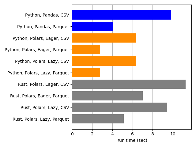
The barplot above shows the processing times for Pandas (blue) and Polars (orange). The gray bars are for Rust, which doesn’t use Pandas, so they aren’t relevant for our comparison.
When we compare “like” to “like”, i.e., when we compare the Python-Pandas-CSV blue bar to the two Python-Polars-CSV orange bars (for Eager and Lazy), it is clear that Polars processing times are lower than Python times. Likewise, the corresponding comparison for the Parquet bars shows that Polars is faster than Pandas. This confirms what we anticipated from those benchmarks.
Python Polars vs. Rust Polars
Our next comparison is between Python-Polars and Rust-Polars.

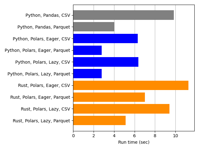
Python-Polars (blue) is faster than Rust-Polars (orange). Since Rust is a compiled language and has a reputation for speed, this is quite surprising.
First, did I do something wrong? That’s entirely possible, since Rust and Polars are fairly new to me. I ensured that Rust compilation times were excluded from the measurement by first running the Rust program a few times manually after compilation to verify that it was optimized and speedy, and then by calling Cargo with the “release” and “frozen” parameters during measurement runs (line 51).
Are they fair comparisons? My purpose was not to write the Python and Rust versions so that they did the exact same lower-level computations. After all, Python and Rust are different languages: I expect that they will do things somewhat differently “under the hood”, even if I write very similar-looking code. My purpose was to write hopefully-straightforward Pythonic and Rustacean code that implemented the same algorithmic ideas without awkward gymnastics to make them exactly the “same”. I think my implementations did that reasonably well. Plus, most of the heavy computational lifting is done by the same library Polars, so that may limit the impact of my particular Pythonic or Rustacean choices. So, I think the comparisons are fair, though someone else might produce fair comparisons that are rather different from mine.
Why is Rust-Polars slower than Python-Polars? Let’s look at the timing measurements in more detail.
path = Path.cwd().parent / 'results'
table_filepath = path / 'min_times_df.csv'
df = pd.read_csv(table_filepath)
df['ratio'] = (df['user_system'] / df['elapsed']).round(2)
df
| program | user | system | elapsed | user_system | ratio | |
|---|---|---|---|---|---|---|
| 0 | s02_python_pandas_csv | 7.44 | 2.11 | 8.51 | 9.84 | 1.16 |
| 1 | s02_python_pandas_parquet | 2.33 | 1.55 | 2.50 | 4.03 | 1.61 |
| 2 | s02_python_polars_eager_csv | 5.43 | 0.77 | 0.70 | 6.31 | 9.01 |
| 3 | s02_python_polars_eager_parquet | 1.99 | 0.55 | 0.50 | 2.78 | 5.56 |
| 4 | s02_python_polars_lazy_csv | 5.39 | 0.57 | 0.73 | 6.37 | 8.73 |
| 5 | s02_python_polars_lazy_parquet | 2.02 | 0.59 | 0.51 | 2.80 | 5.49 |
| 6 | s02_rust_polars_eager_csv | 10.18 | 0.85 | 1.46 | 11.28 | 7.73 |
| 7 | s02_rust_polars_eager_parquet | 6.12 | 0.66 | 1.21 | 7.00 | 5.79 |
| 8 | s02_rust_polars_lazy_csv | 8.28 | 0.87 | 0.95 | 9.42 | 9.92 |
| 9 | s02_rust_polars_lazy_parquet | 4.14 | 0.78 | 0.68 | 5.13 | 7.54 |
Notice that the sum of the user and system times exceeds the elapsed times for both Python-Polars and Rust-Polars. This suggests that Polars is parallelizing its workload (“embarrassingly parallel“). The ratios for user+system:elapsed are sometimes higher for Rust-Polars than for Python-Polars — specifically for the Lazy variations. Does Rust-Polars incur more overhead for parallelization operations than Python-Polars even while the workload isn’t heavy enough to justify this extra cost? That’s an interesting hypothesis. But the differences in the ratios aren’t that large, and small fluctuations in the small elapsed denominators could alter the ratios substantially. Additionally, the ratios for the Eager cases either favor Python or are virtually identical, so we would need a better explanation that might account for both Eager and Lazy comparisons between the languages.
A deeper investigation might involve line-profiling the Python and Rust variations of each comparison to locate the most time-consuming operations. Absent that closer look, I would recommend not just assuming (as I did) that one language would be faster than another for a particular use case: if optimization for speed is that important, it’s worth testing the alternatives to know for sure.
CSV vs. Parquet
Next we compare reading data from CSV files to reading from Parquet files.

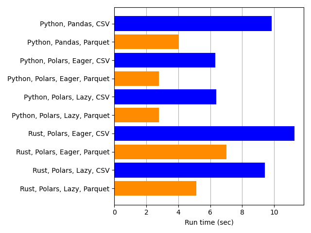
This comparison turned out as expected: loading data from Parquet files (orange) is faster than reading CSV files (blue). And that was true for every comparison pair: Python-Pandas, Python-Polars-Eager, Python-Polars-Lazy, Rust-Polars-Eager, and Rust-Polars-Lazy.
One feature of Parquet files that surely makes them faster in this case is that they store data as columns, meaning that values that are adjacent in a column are also adjacent in the file structure or in memory when they are read. By contrast, CSV files store data in rows. When only a subset of columns are loaded from a file, read times from Parquet are often fast because of this column-based storage.
Polars Eager vs. Polars Lazy
Finally we compare eager versus lazy execution in Polars.

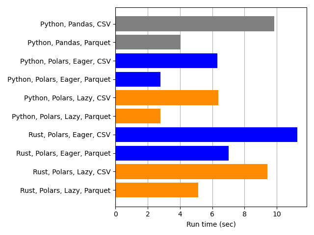
There’s no discernible difference between eager (blue) and lazy (orange) Polars execution with the Python code. This would make me question whether I completely botched coding the Lazy implementation, except that for Rust, Lazy is indeed faster than Eager for both CSV and Parquet. That’s reassuring; I must’ve done something right.
Why is Lazy faster than Eager for Rust but not for Python? Perhaps Rust’s compiler allows optimizations between Polars’s Lazy execution mode and other Rust code that the Python interpreter can’t do. A similar improvement in Python might require a lot of manual investigation and optimization effort.
Conclusion
For the most part, the results were as I expected: Polars is faster than Pandas, Parquet is faster than CSV, and Lazy is faster than Eager.
The major exception was that Python-Polars was faster than Rust-Polars when I expected that Rust would be faster than Python. On the one hand, a computer scientist might scoff at the difference because it’s less than an order of magnitude; in fact, Rust is more than 2-times slower than Python in only one case, and even that is only 2.5-times slower:
rust_to_python_ratios = [
    (df['program'].iloc[i],
     df['program'].iloc[i+4],
     df['user_system'].iloc[i+4] /
     df['user_system'].iloc[i])
    for i in range(2, 6)]
ratio_df = pd.DataFrame(rust_to_python_ratios)
ratio_df.iloc[:, -1] = ratio_df.iloc[:, -1].round(2)
ratio_df
| 0 | 1 | 2 | |
|---|---|---|---|
| 0 | s02_python_polars_eager_csv | s02_rust_polars_eager_csv | 1.79 |
| 1 | s02_python_polars_eager_parquet | s02_rust_polars_eager_parquet | 2.52 |
| 2 | s02_python_polars_lazy_csv | s02_rust_polars_lazy_csv | 1.48 |
| 3 | s02_python_polars_lazy_parquet | s02_rust_polars_lazy_parquet | 1.83 |
On the other hand, a factor of 2 or 3 can provide important time savings in real-world applications, so optimizing for such a difference might be worthwhile.
Further investigation should focus on whether some minor adjustments to the Rust code would greatly improve its performance or whether Python has a general advantage for this type of data processing with Polars.
