
Ways to get more out of your models
Full Bayesian vs. Quantile Regression: Linear Data
When we need our models to produce a full posterior distribution for our predictions, we can bring to bear the full suite of tools from Bayesian analysis. Sometimes, though, we need shortcuts: using the full Bayesian model may exceed our computational limitations, or we may not have the tooling and infrastructure to readily productionize it. In such cases, quantile regression can be a convenient alternative.
Quantile regression lets us predict a chosen quantile (e.g., the median, the 80th percentile) of our predicted outcome variable’s distribution. This distribution isn’t exactly the same as the predicted posterior distribution of a full Bayesian model, because it doesn’t account for a prior. However, in cases where the prior is very weak or the large number of cases in our data set lets the likelihood overwhelm the prior’s effects on the posterior, the predicted quantiles can be reasonably close to the corresponding positions of the posterior.
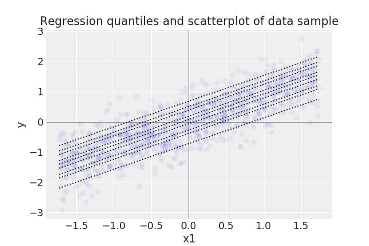
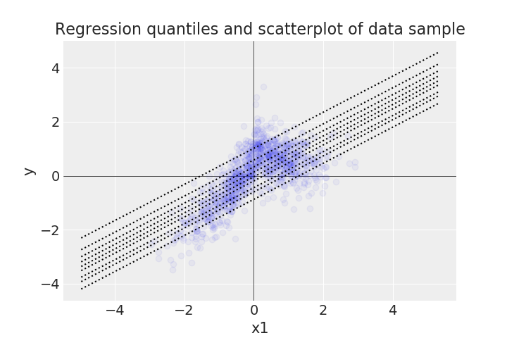
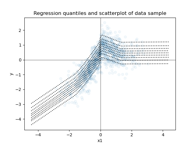
To illustrate this similarity, I generated some positively correlated bivariate data with Gaussian noise in the response variable, so that I could run some simple regression models on it. Below is a scatterplot of a sample of the data along with every decile (from the 10th to the 90th) of the predicted posterior distribution of a full Bayesian linear model with weak priors on its parameters.
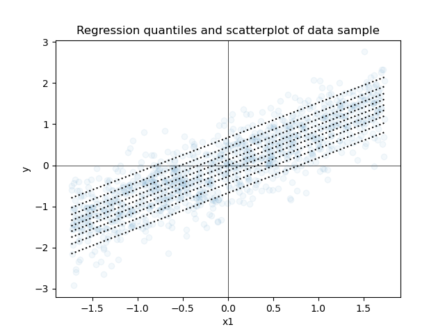
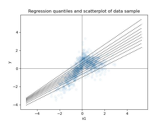
Next is a scatterplot of the same data along with every decile from quantile regression models, where each model predicts a single decile.
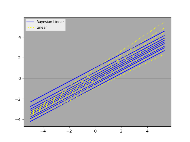
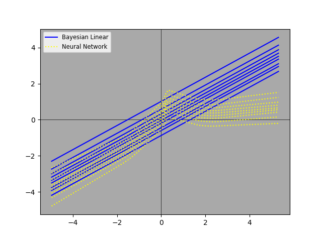
The two plots appear to be very similar. We can juxtapose the Bayesian and non-Bayesian predictions on a single plot, so that we can compare them more carefully.
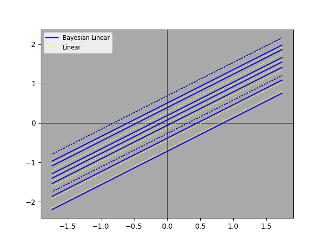
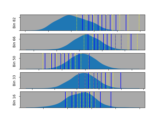
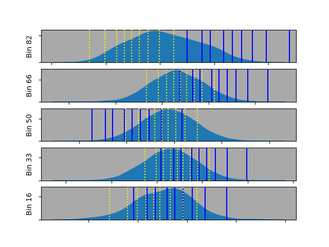
The two sets of predictions aren’t identical, but they’re quite close. We can also look at slices along the x-axis, so that we can see the distributions and the two sets of predictions. For this purpose, we group the data into 100 bins and show just a few bins along the x-axis.
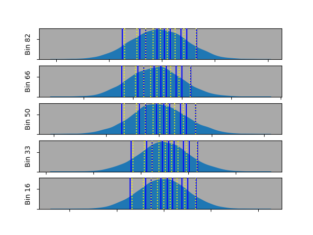
The density plots show the Gaussian-distributed noise along the y-axis for each bin. Accordingly, we can now see the distribution and its predicted deciles together.
Full Bayesian vs. Quantile Regression: Curvy Data
The data for our examples above was generated from a linear model, so the Bayesian linear regression and quantile linear regression models readily fit to the data very well. But we often have data that is more complicated, so our first attempt at fitting a linear model might not work so well. Here’s an example of Bayesian linear regression predictions on a curvier data set.
And here’s the quantile regression predictions for the same data.
And here they are superimposed.
Clearly, the linear models are having difficulties. Noticeably, the quantile regression models choose slopes so that the predictions of the deciles separate, or fan out, as one looks from low x-values (left) to high x-values (right). That diverging adjustment might mean that each adjacent pair of deciles actually does bound ~10% of the data points overall, but those are clearly poor predictions conditional on x. We can see this even more clearly below where the Gaussian distributions and the decile predictions markedly diverge for several bins.
Of course, this isn’t surprising. If we really want our linear models to fit non-linear data, we should make them more flexible by, for example, adding polynomial terms or (when we have >1 predictor) interaction terms or the like.
An alternative is to use more flexible modeling algorithms like tree ensembles or neural networks. The Python package scikit-learn has some convenient methods for doing this, but I chose to create my own implementation in PyTorch.
While we can continue to create one model per predicted quantile it might be more efficient for both training and inference to incorporate all the predicted deciles into a single model. We can do this with multi-task learning.
Here are the results from one training run of the model:
Clearly, the more flexible neural network model is adhering more closely to the deciles condtional on x. We can also see this when we compare the results to the Bayesian linear regression decile predictions.
While the neural network results aren’t perfect, they clearly track the Gaussian distribution in each x-bin more closely than the linear results do.
Summary
In summary, we sometimes want more information from our model than just a single point estimate of the response variable’s mean or median; we might want to know more about the broader range of the prediction. Bayesian models with informative priors are often our best solution, because they can provide us with a full posterior predictive distribution. But they do have their drawbacks, including computational intensity. So a “compromise” solution might be quantile regression, which we implemented for a linear model and for a more flexible neural network.