If you prefer a prettier rendering of the code and dataframes displayed in this article, you are welcome to read the notebook at my Github repo.
How to add columns to Polars dataframes fast
The Conundrum
I was recently writing a function to add columns of moving averages to a Polars dataframe. For a particular problem, this is a simple thing to do. For example, we might have a dataframe like this (line 17 for a similar example):
import warnings
import datetime
import polars as pl
warnings.filterwarnings('ignore')
df = pl.DataFrame({
    'timestamp': [
        datetime.datetime(2022, 2, 1, 10, 0, 0),
        datetime.datetime(2022, 2, 1, 10, 0, 1),
        datetime.datetime(2022, 2, 1, 10, 0, 2),
        datetime.datetime(2022, 2, 1, 10, 0, 3),
        datetime.datetime(2022, 3, 1, 10, 0, 4)],
    'data': [1, 2, 3, 4, 5]})
df
| timestamp | data |
|---|---|
| datetime[μs] | i64 |
| 2022-02-01 10:00:00 | 1 |
| 2022-02-01 10:00:01 | 2 |
| 2022-02-01 10:00:02 | 3 |
| 2022-02-01 10:00:03 | 4 |
| 2022-03-01 10:00:04 | 5 |
Suppose we want to add three columns of moving averages, one with a window size of 2, the second window of size 3, and the final one of size 4. That’s a straightforward command in Polars (line 85):
def calculate_moving_averages_hard_coded(
    df: pl.DataFrame, data_colname: str='data') -> pl.DataFrame:
    """
    Calculates moving averages of 'data_colname' column in dataframe 'df' with
        3 window sizes, so that each window size corresponds to a single column
        of moving averages
    """

    mas_df = df.with_columns(
        ma_2=pl.col(data_colname).rolling_mean(window_size=2),
        ma_3=pl.col(data_colname).rolling_mean(window_size=3),
        ma_4=pl.col(data_colname).rolling_mean(window_size=4))

    return mas_df
result = calculate_moving_averages_hard_coded(df)
result
| timestamp | data | ma_2 | ma_3 | ma_4 |
|---|---|---|---|---|
| datetime[μs] | i64 | f64 | f64 | f64 |
| 2022-02-01 10:00:00 | 1 | null | null | null |
| 2022-02-01 10:00:01 | 2 | 1.5 | null | null |
| 2022-02-01 10:00:02 | 3 | 2.5 | 2.0 | null |
| 2022-02-01 10:00:03 | 4 | 3.5 | 3.0 | 2.5 |
| 2022-03-01 10:00:04 | 5 | 4.5 | 4.0 | 3.5 |
But what if we don’t know the window sizes in advance, or even how many columns of moving averages we want to add? It would be better to pass the window sizes as a parameter to the function. That way, our function can accommodate any number and any sizes of windows.
However, I found myself scratching my head about how to best do this in Polars. It would be easy to add each column one-by-one in a loop. But a big reason to use Polars instead of other dataframe libraries is that Polars is fast, partly because it can parallelize its workloads. It can’t parallelize creating our moving-average columns if we’re creating only one column at a time.
I figured Polars had something that would handle this conundrum — maybe an apply method that would work across columns instead of rows. But I didn’t find anything. There might very well be something obvious that I missed; and the Polars API is rapidly evolving, so if a feature doesn’t exist now, it likely will soon. In any case, I found a good solution when I started thinking beyond the Polars API.
A Possible Solution
I started thinking about how I used to generate SQL queries as Python strings, which saved me a lot of tedious typing when I had to specify a multitude of conditions as CASE statements. Could we do the same thing here?
Yes, we can. Python has exec and eval functions that let us execute a string as Python code. For example, we can create a list like this:
a_list = eval('["meow", "bark", "oink", "moo"]')
a_list
['meow', 'bark', 'oink', 'moo']
Or do some arithmetic:
a_sum = eval('4 + 3')
a_sum
7
Okay, that means that we can dynamically construct a Polars command to add as many moving-average columns to our dataframe as we want. But will that approach actually be faster? Let’s test it and see.
Solution Code
First, we need to generate some data. We can simply create a dataframe with a series of timestamps and some Gaussian-distributed data. We’ll later calculate the moving averages on that Gaussian data (line 50).
import numpy as np
def generate_data(
    start_datetime: datetime.datetime=datetime.datetime(1970, 1, 1, 0, 0, 0),
    end_datetime: datetime.datetime=datetime.datetime(1970, 1, 1, 0, 1, 0),
    interval: str='1s',
    column_n: int=1):
    """
    Generates of Polars DataFrame with a 'timestamp' column and a provided
        number ('column_n') of columns of standard-normally distributed data
    For acceptable input values for 'interval', see:
        https://pola-rs.github.io/polars/py-polars/html/reference/expressions/api/polars.date_range.html
    """

    timestamp = pl.date_range(
        start_datetime, end_datetime, interval, eager=True).alias('timestamp')

    data = [
        pl.Series(np.random.normal(size=len(timestamp))).alias(f'data{i}')
        for i in range(column_n)]

    df = pl.concat(
        [pl.DataFrame(timestamp), pl.DataFrame(data)], how='horizontal')

    return df
start_datetime = datetime.datetime(2020, 1, 1, 0, 0, 0)
end_datetime = datetime.datetime(2020, 2, 1, 0, 0, 0)
interval = '1s'
data_column_n = 1
df = generate_data(start_datetime, end_datetime, interval, data_column_n)
df.head()
| timestamp | data0 |
|---|---|
| datetime[μs] | f64 |
| 2020-01-01 00:00:00 | -1.401879 |
| 2020-01-01 00:00:01 | 0.23502 |
| 2020-01-01 00:00:02 | -2.305322 |
| 2020-01-01 00:00:03 | -1.373878 |
| 2020-01-01 00:00:04 | -0.188347 |
An example of the generated data is above.
Next we need a function that will calculate each column of moving averages one by one (line 93).
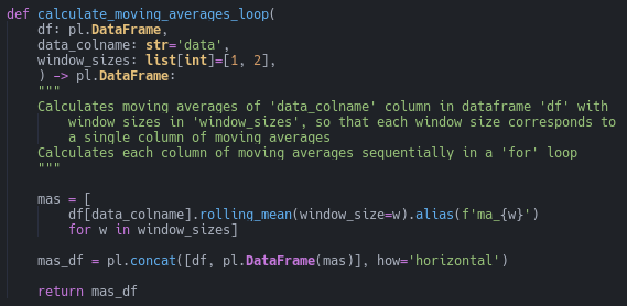
Notice that the columns are calculated sequentially in the list comprehension. Then they’re all assembled into the dataframe together.
Now we need a function that implements our hopefully-faster solution: constructing a Polars command that includes all our columns as a string, then executing it all at once (line 114).
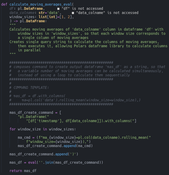
Notice that the loop now adds a string for each column, instead of actually executing a command to create each column as in our prior function. The final execution is handled by Python’s eval function.
Finally, it’ll be convenient to have a function that records how fast our two approaches are (line 157).
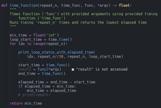
We can call our timing function like this (line 215):

Notice that we send both the function that we want to time and the function that does the timing (perf_counter, in this case) to our timing function.
Timing Conditions
For our testing scenario, I set 200 different window sizes (line 205), so that 200 columns of moving averages would be added to the dataframe. I ran each test condition 400 times (line 211) and used the lowest recorded time. There were two types of times measured: the elapsed time, or wall-clock time and the system+user time, that is, the sum of the reported system time and the user time. During timing runs, my machine wasn’t running any web browsers, multimedia players, or other processing-intense applications, and I watched the system monitor to verify that no unexpected processes were using substantial system resources.
Timing Results
The timing results clearly show that constructing the string query to be executed all at once by Polars is faster than creating each moving average column one-at-a-time. Judging from the elapsed time, the String Query, Eval approach is about 6 times faster than the Loop One-by-One method.
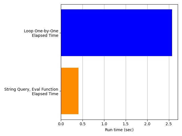
Also, Polars is clearly accelerating the String Query, Eval approach by parallelizing the workload. Look at the next plot, which repeats the elapsed times in the plot above and adds the system+user time. The two times for the Loop One-by-One approach (blue bars) are nearly the same, suggesting that the processing is all serial. But the system+user time for the String Query, Eval approach is much higher than the elapsed time (orange bars), suggesting that a lot more processing is getting crammed into that small elapsed time — that is, the workload is being parallelized.
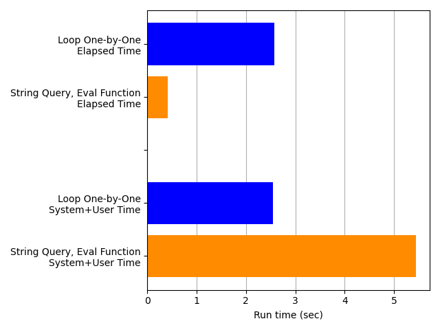
This conclusion is consistent with my observations of my computer’s CPU usage: the String Query, Eval code was clearly engaging multiple cores simultaneously, while the Loop One-by-One code did not.
This is good news: the String Query, Eval approach works faster, exactly as intended. However, it does have some disadvantages that we want to consider before choosing it.
Disadvantages of the String Query, Eval Approach
One disadvantage of the String Query, Eval approach is that it doesn’t play nicely with IDEs like NeoVim or VSCode. Take a closer look at the signature for our function that uses eval.

Notice that the Language Server Protocol (LSP) claims that we didn’t use the parameters df and data_colname in our function. But we did. We put them inside a string, so the LSP can’t detect them (I’m using Pyright in an IDE built on Neovim).

By contrast, notice that the LSP has no such difficulty detecting the same variables in our Loop One-by-One function.

Another IDE-relevant disadvantage is that the String Query, Eval function is less readable, because the code inside the string doesn’t benefit from syntax highlighting.
A more serious issue is that using the Python exec and eval functions can be a security vulnerability. If a nefarious actor could provide or alter our string query, they could make our computer system execute any code that could compromise our security, much like a SQL injection attack.
In this particular case, though, that attack method isn’t a great concern. We’re hard-coding our string (except for the values of our variables) within our function, and we’re not accepting any string input from outside parties. If a nefarious actor could alter our string, they also have enough access to alter any of our code; the query string is no more vulnerable than the rest of our code. So while our code is quite safe for our timing exercise here, this security vulnerability would be a serious concern in most production systems.
Conclusion
To summarize, constructing a string query that is submitted to Polars so that all our moving-average columns are created at once is a fast and viable alternative to creating each column one-by-one. So long as security issues are not a concern, the only remaining trade-off against performance is code readability in the IDE. But the best alternative would be to find a way to do this within the Polars API: that way, we could enjoy both performance and readability.
